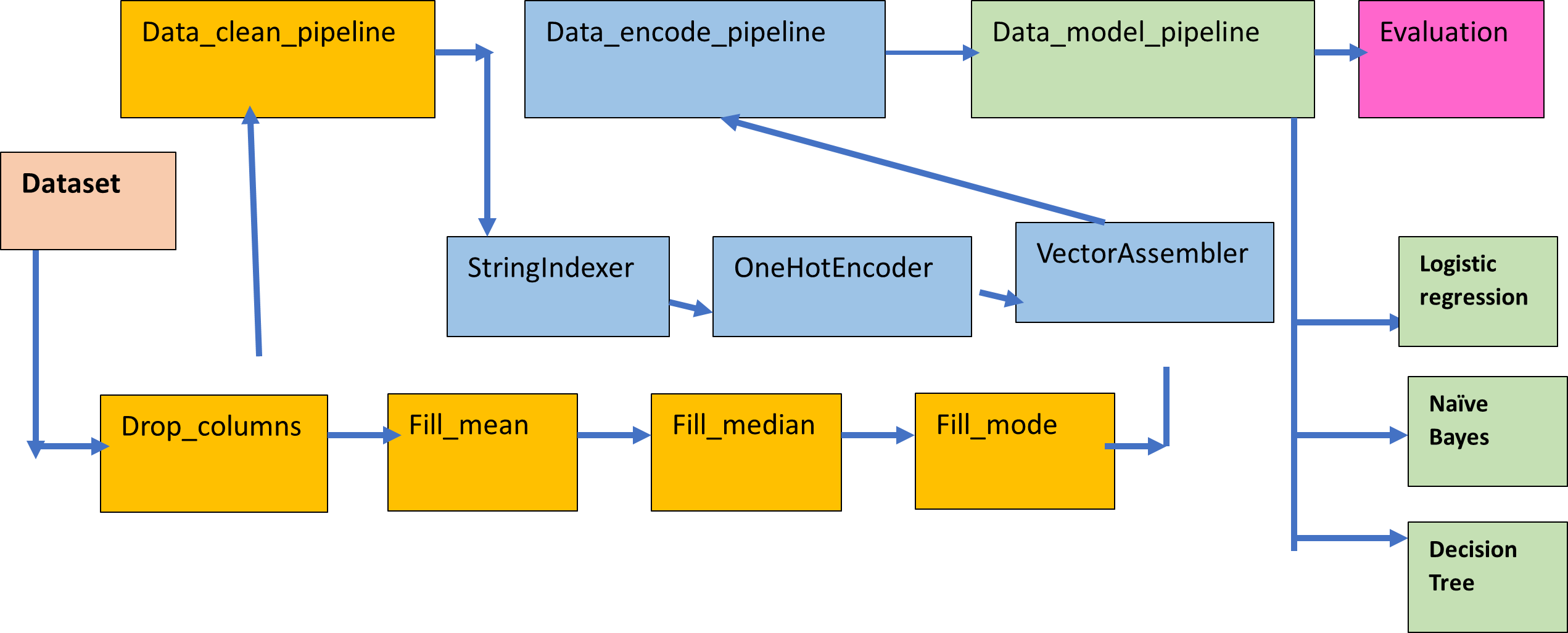
In this article I am going to illustrate the process to perform machine learning classification in Pyspark with Pipeline. A pipeline is a sequence of stages used to perform a specific task. In the pipeline , the output of a task in a stage acts as an input to the next stage of the pipeline. The machine learning pipeline is composed of multiple stages, like data cleaning, filling of missing values, encoding, modelling and evaluation. The pipeline is a more organised and structured way to code and a machine learning pipeline helps to speed up the process by automating the workflows and synchronizing them together.
What is Bigdata?
Big data refers to vast, complex datasets from various sources, including social media, sensors, and more. The features of these complex datasets can be referred to as the 5 V’s:-
Volume: It’s massive, often terabytes to exabytes, beyond traditional systems. The companies which process or analyze huge numbers of transactions per unit time e.g. Walmart falls in this category
Velocity: Data is generated in high speed like social media data or sensor data
Variety: It’s diverse, from structured databases to unstructured text and images.
Veracity: Dealing with uncertain or unreliable data quality. The data available from the web is noisy and chaotic, comprising of missing values or inconsistent data.
Value: Extracting insights for data-driven decisions. The data can generate valuable business insights required to take important decisions or provide Business intelligence.
Tools like Hadoop, Spark, NoSQL databases, and machine learning help analyze big data for industries like business, healthcare, finance, and marketing.
Introduction to Spark
Spark is an open source Bigdata analytics framework which started in 2009 as a small project in Berkeley’s lab to improve the performance of Hadoop. Spark uses in-memory computation in contrast to Hadoop which write all the temp files in the persistent storage. Due to the in-memory computation , Spark is 100 times faster than Hadoop Map reduce. Spark emerged as an Apache popular Project in February, 2014.
Spark does not have its own storage, It can use Hadoop HDFS , AWS, GCP or any other cloud storage. Spark provides an user friendly API in multiple programming languages like Python, Scala, R and Java.
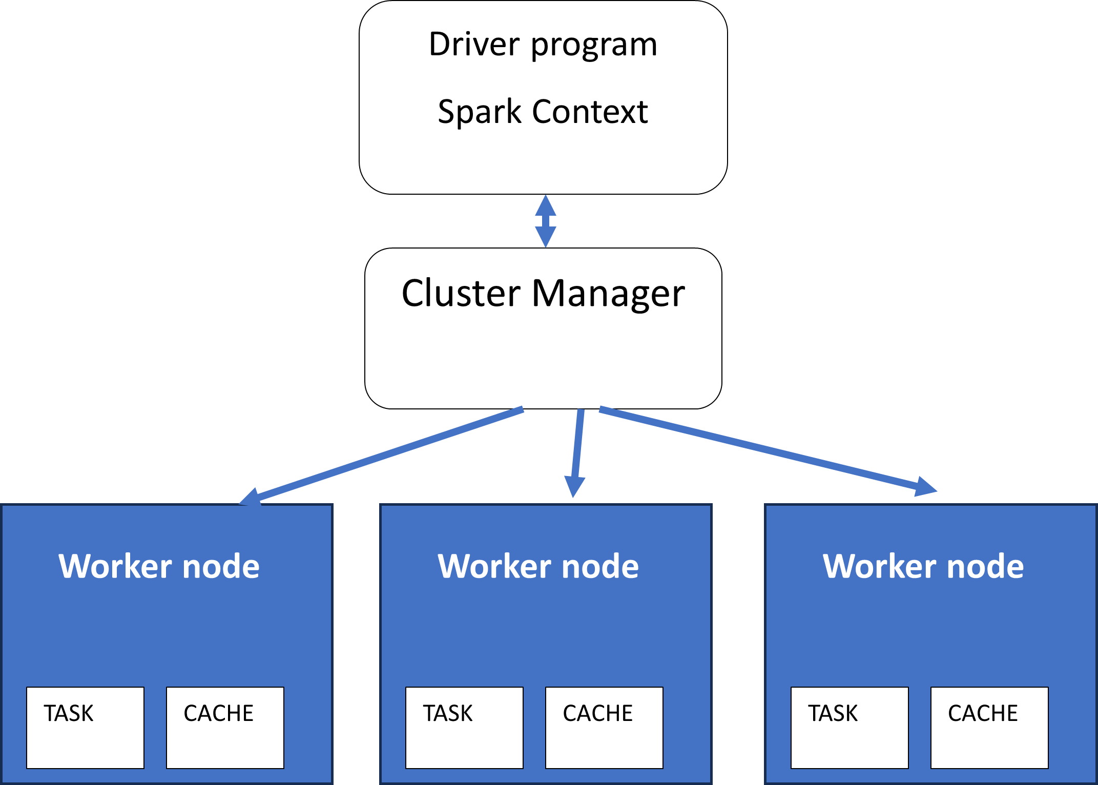
SparkContext
Spark has a master slave architecture. It has a master node or Driver which acts as a coordinator for multiple worker nodes or executors which perform actual processing on the data. SparkContext (sc) is the entry point to work with the master node of the Spark or Spark Driver. It is used to create RDDs (Resilient Distributed datasets) which are chunks of immutable datasets formed by partitioning the Datasets imported in Spark. Parallel processing is performed on RDDs where-ever possible for generating summarisations. In Spark , the SparkContext or SC is automatically generated by the environment. In Pyspark, the SparkContext need to be initialized explicitly.
Spark
The spark variable is the entry point to the Spark Data Frame API. It can be created as an instance of the SparkSession. The Spark variable can be used to execute SQL queries in Spark.
click on thumbnail to open the full image
Pyspark
Pyspark is a Python API available to work with Spark. One need to import the pyspark module in Python and then create the environment for working with the Spark framework. The instances of SparkContext and SparkSession need to be created explicitly with Python code. For successful working of pyspark, Spark should be installed in your machine and pyspark should also be installed , which has the same version as your Spark shell installed in your machine.
Dataset
The dataset used is titanic dataset from kaggle. It has both train and test datasets
https://www.kaggle.com/competitions/titanic/data
Importing libraries
#basic libraries for data preprocessing
import pyspark
import numpy as np
import pandas as pd
import seaborn as sns
from pyspark.sql import DataFrame
#data preparation libraries
from pyspark.ml.feature import StandardScaler,PCA
from pyspark.ml.feature import StringIndexer,OneHotEncoder,VectorAssembler
#libraries for machine learning classification
from pyspark.ml.classification import LogisticRegression,DecisionTreeClassifier,NaiveBayes,RandomForestClassifier
#library for evaluation for calculating accuracy_score, precision,recall
from pyspark.ml.evaluation import BinaryClassificationEvaluator
#machine learning pipeline
from pyspark.ml import Pipeline
from pyspark.ml import Transformer #for creating custom classes for pipeline
#libraries for creating spark environment
from pyspark import SparkContext
from pyspark.sql import SparkSession
#creating spark environment
sc=SparkContext() #creating an instance for sparkcontext, entry point for spark
spark=SparkSession.builder.master(“local[1]”).appName(“titan”).getOrCreate() #entry point for Spark dataframe API
#importing csv file
df_tr=spark.read.option(“header”,True).option(“inferSchema”,True).csv(“c:/csv-ml/titanic_train.csv”)
df_test=spark.read.option(“header”,True).option(“inferSchema”,True).csv(“c:/csv-ml/titanic_test.csv”)
#checking missing values
df_tr_pd=df_tr.toPandas()
df_test_pd=df_test.toPandas()
df_tr_pd.isna().sum()
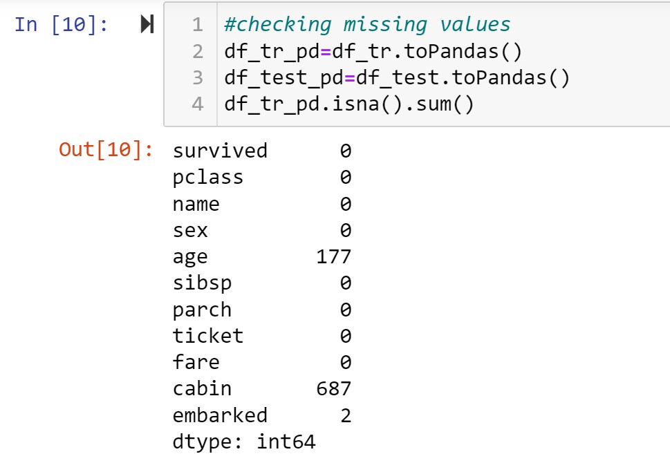
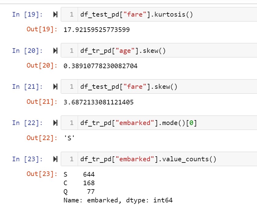
Age,Cabin and embarked have missing values. By analysing the data , it is observed that cabin consists of mostly unique elements and that too a list of cabin numbers and I decided to drop the columns name,ticket and cabin. For age , fare and embarked I performed univariate analysis and decided to replace them by mean,median and mode respectively.
Age column is normally distributed while fare column is right skewed while the embarked column is a categorical variable. Fare column has missing values in the test dataset. Performed these preprocessing steps by pipeline method.
Univariate analysis of the columns having missing values
Creating custom transformers for the pipeline
#a transformer which drops the specific columns
class ColumnDropper(Transformer):
“””
A custom Transformer which drops all columns
“””
def __init__(self, banned_list):
self.banned_list = banned_list
def _transform(self, df: DataFrame) -> DataFrame:
for i in self.banned_list:
df=df.drop(i)
return df
#a transformer which fills missing values with mean
class Columnfiller_mean(Transformer):
“””
A custom Transformer which drops all columns
“””
def __init__(self,col):
self.col = col
def _transform(self, df: DataFrame) -> DataFrame:
m=df.agg({self.col:”avg”}).collect()[0][0]
df=df.fillna(value=m,subset=[self.col])
return df
#a transformer which fills missing values with median
class Columnfiller_median(Transformer):
“””
A custom Transformer which drops all columns
“””
def __init__(self,col):
self.col = col
def _transform(self, df: DataFrame) -> DataFrame:
q=df_tr.approxQuantile(“fare”, [0.5], 0.0) #fills with 50% ,2nd quartile or median
str_quant=””.join(str(q[0])) #converts the list format to string
quant=float(str_quant) #converts string to float which fills the missing values
df=df.fillna(value=quant,subset=[self.col])
return df
#a transformer which fills missing values with mode
class Columnfiller_mode(Transformer):
“””
A custom Transformer which drops all columns
“””
def __init__(self,col):
self.col = col
def _transform(self, df: DataFrame) -> DataFrame:
m=df.agg({self.col:”max”}).collect()[0][0] #value with maximum frequency
df=df.fillna(value=m,subset=[self.col])
return df
#creating the stages of the data preparation pipeline
stage1_clean=ColumnDropper(banned_list = [“cabin”,”ticket”,”name”])
stage2_clean=Columnfiller_mean(“age”)
stage3_clean=Columnfiller_median(“fare”)
stage4_clean=Columnfiller_mode(“embarked”)
pipeline_clean=Pipeline(stages=[stage1_clean,stage2_clean,stage3_clean,stage4_clean])
#creating the stages of the data encoding pipeline
#stage1 performs label encoding of the categorical columns
stage1_encode=StringIndexer(inputCols=[‘sex’,’embarked’],outputCols=[‘sex_idx’,’embarked_idx’])
#stage2 performs one hot encoding on the label encoded columns
stage2_encode=OneHotEncoder(inputCols=[‘sex_idx’,’embarked_idx’],outputCols=[‘sex_ohe’,’embarked_ohe’])
#stage3 creates a single feature vector by combining the numeric columns and one hot encoded columns
stage3_encode=VectorAssembler(inputCols=[‘pclass’, ‘sex_ohe’, ‘age’, ‘sibsp’, ‘parch’, ‘fare’, ’embarked_ohe’],outputCol=”features”)
pipeline_encode=Pipeline(stages=[stage1_encode,stage2_encode,stage3_encode])
#fitting the data preparation pipelines
#clean the training dataset
df_clean=pipeline_clean.fit(df_tr).transform(df_tr)
df_final=pipeline_encode.fit(df_clean).transform(df_clean)
#clean the test dataset
df_clean_test=pipeline_clean.fit(df_test).transform(df_test)
df_final_test=pipeline_encode.fit(df_clean_test).transform(df_clean_test)
#selecting the features to be used with model, we need the feature vector and target variable
df_final2=df_final.select(“features”,”survived”)

#splitting the dataset
tr,test=df_final2.randomSplit([.75,.25],seed=100)
#creating predictive modelling pipeline
#the pipeline first perform z-score normalization followed by predictive modelling
#logistic regression
logit_pipeline=Pipeline(stages=[StandardScaler(inputCol=”features”,outputCol=”features_scaled”),LogisticRegression(featuresCol=”features_scaled”,labelCol=”label”)])
#naive bayes classification
naive_pipeline=Pipeline(stages=[StandardScaler(inputCol=”features”,outputCol=”features_scaled”), NaiveBayes(featuresCol=”features_scaled”,labelCol=”label”)])
#decision tree classification
dtree_pipeline=Pipeline(stages=[StandardScaler(inputCol=”features”,outputCol=”features_scaled”),DecisionTreeClassifier(featuresCol=”features_scaled”,labelCol=”label”)])
#creating model pipeline
model_pipeline=[logit_pipeline,naive_pipeline,dtree_pipeline]
#creating instance of the evaluator
eval=BinaryClassificationEvaluator(labelCol=”label”,rawPredictionCol=”prediction”,metricName=”areaUnderROC”)
#fitting the data to the models in a loop to determine training accuracy
model_fit=[] #list to store fitted models
for i in model_pipeline:
j=i.fit(tr).transform(tr) #predicting with training dataset
model_fit.append(j)
#creating the dataframe
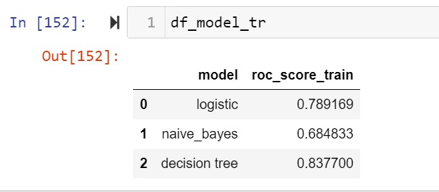
df_model_tr=pd.DataFrame({“model”:[“logistic”,”naive_bayes”,”decision tree”],”roc_score”:eval_mod})
#prediction with the validation dataset
model_fit_test=[]
eval_mod_test=[]
for i in model_pipeline:
j=i.fit(tr).transform(test) #fitting with tr and prediction with test
eval_mod_test.append(eval1.evaluate(j)) #evaluation
model_fit_test.append(j)
#test score
df_model_test=pd.DataFrame({“model”:[“logistic”,”naive_bayes”,”decision tree”],”roc_score_test”:eval_mod_test})
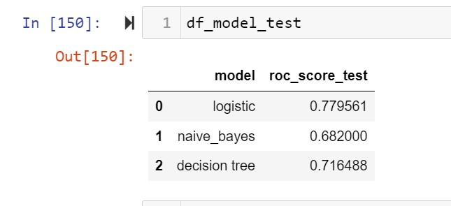
The logistic regression model shows minimum overfitting so selecting that model for predicting the test dataset
#prediction with actual test dataset
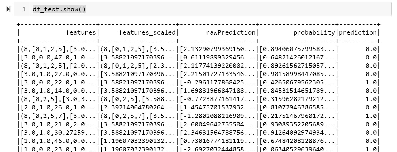
df_final_test2=df_final_test.select(“features”)
df_test=logit_pipeline.fit(df_final2).transform(df_final_test2)
df_test.show()